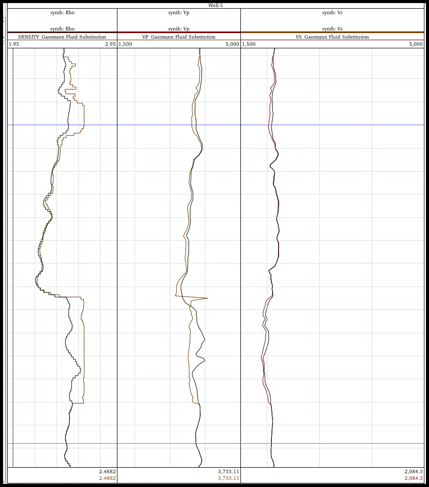
Gassmann Fluid Substitution
This process calculates new density, P-velocity, and S-velocity curves using the Gassmann Equation. Gassmann is an equation to derive P-velocity, S-velocity and density in a rock medium in which the original fluid was replaced by another fluid (fluid substitution).
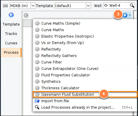
- In the Control Panel, go to View > New Single Well View.
- In the Single Well window, open the Process tab.
- At the tab header, click the blue "+" icon.
- Click Gassmann Fluid Substitution.
- Type a name for the process and click OK.
Configure the Gassmann Fluid Substitution process
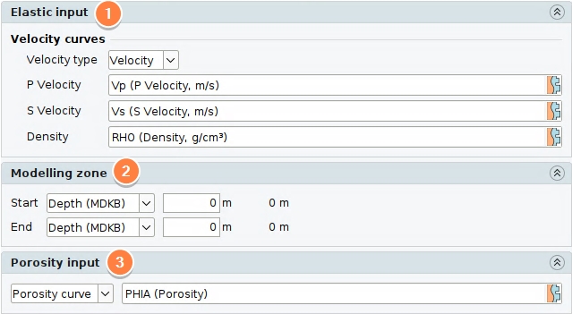
- Elastic input
- Velocity curves:
- Velocity type:
- Velocity: Select to calculate from velocity curves.
- Slowness: Select to calculate from sonic logs (slowness).
- Curve selection: Choose a curve for each entry (P Velocity or P Slowness, S Velocity or S Slowness, Density). The available Vp/Vs curves depend on the chosen velocity type.
- Velocity type:
- Velocity curves:
- Modelling zone: Set the Start and End of the interval over which to perform the fluid substitution. For each boundary, select the reference type from the dropdown:
- Top of well: Uses the shallowest measured depth of the well (minimum MD) as the base. An optional offset (in project units) can be added. The resulting depth is displayed alongside the field.
- TD of well: Uses the total depth of the well (maximum MD) as the base. An optional offset (in project units) can be added. The resulting depth is displayed alongside the field.
- Depth (MDKB) or Depth (TVDSS/TVDBML): Enter a depth value directly in the chosen depth domain.
- Horizon: Select a horizon from the project. The depth is derived from the horizon's intersection with the well.
- Marker: Select a marker (well top) from the well.
- Porosity input: Specifies how porosity is provided for the calculation. Select one of three options from the drop-down:
- Porosity curve: Select a porosity curve as the input.
- Density curve: Select to derive porosity from the density curve using the density-porosity equation:
φ = (ρgrain − ρbulk) / (ρgrain − ρfluid)
where ρbulk is the density curve value, ρgrain is the composite matrix density (see Mineral info), and ρfluid is the in-situ pore fluid mixture density (water and hydrocarbon densities weighted by the in-situ water saturation, see Gassmann substitution scenarios). - Constant value: Specify a single constant porosity value (%) to use across the reservoir interval.
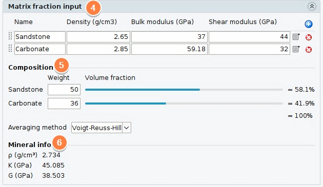
- Matrix fraction input: Define one or more minerals that make up the rock matrix. Each mineral has:
- Name: A label for the mineral (e.g. Quartz, Calcite, Clay).
- Density (g/cm³): Density of the mineral.
- Bulk modulus (GPa): Bulk modulus of the mineral.
- Shear modulus (GPa): Shear modulus of the mineral.
- Preset: Quickly populate density, bulk modulus, and shear modulus from a preset mineral types (Sandstone, Limestone, Carbonate, and Claystone)
Minerals can be added using the blue (+) button and removed using the red (x) button. At least one mineral must remain.
-
Composition:
-
Weight: Specify the relative weight of each mineral.
-
Volume fraction: A bar showing each mineral's fraction normalised to 100%. Adjust the Weight values to change the composition.
-
Averaging method: Select either Voigt-Reuss-Hill or Reuss averaging method.
-
-
Mineral info: Dynamically displays the calculated composite matrix properties—density (ρ), bulk modulus (K), and shear modulus (G).
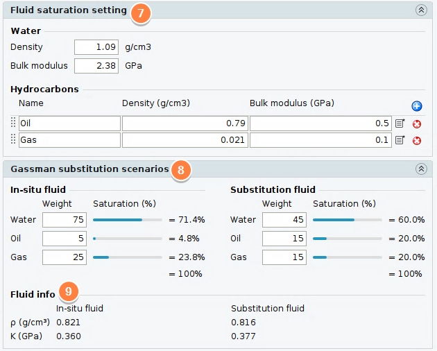
- Fluid saturation setting: Defines the fluid phases used in the substitution.
- Water: Specify the properties of the water phase:
- Density (g/cm³): Density of water.
- Bulk modulus (GPa): Bulk modulus of water.
- Hydrocarbons: Define one or more hydrocarbon fluid phases. Each phase has:
- Name: A label for the fluid phase (e.g. Oil, Gas, Condensate).
- Density (g/cm³): Density of the fluid phase.
- Bulk modulus (GPa): Bulk modulus of the fluid phase.
- Preset: Quickly populate density and bulk modulus from a built-in preset (Oil, Gas, Condensate, Heavy oil).
- Water: Specify the properties of the water phase:
- Gassmann substitution scenarios: Specify the relative saturation of water and hydrocarbon phases. Alongside each entry, a bar shows the weight normalised to 100%.
- In-situ fluid: The expected relative saturation of water and hydrocarbon fluid phases in the recorded well data.
- Substitution fluid: The relative replacement saturation of water and the hydrocarbon fluid phases.
-
Fluid info: Displays the input density (ρ) and bulk modulus (K) values for both the original in-situ fluid and the target substitution fluid.

- Output
- Curves
- Enable custom name: Specify the name of the output curves. Each curve will be named as "[output class]_[process name]" by default, or if a custom name is supplied, "[output class]_[custom name]".
- Extent: Specify the extents of the output curves.
- Curves